What is the Vlookup in Excel?
VLOOKUP is a function commonly used to find or retrieve data in Excel. It is used to search for a specific value in a table and returns a corresponding value from another column. This function is extensively utilized when you need to look up and extract data from a large dataset.
Before using the VLOOKUP function, it is necessary to understand what this function is and why it is used in Excel. As you may know, Microsoft Excel has various types of formulas, and the VLOOKUP function is used to search for a value in Excel or to retrieve data from a table, workbook, or worksheet.
Syntax: VLOOKUP(lookup_value, table_array, col_index_num, [range_lookup])
VLOOKUP V” stands for “vertical” | Default: [range_lookup]=True
Vlookup Formula in Excel with Example:
let’s understand the syntax of the VLOOKUP function with some examples so that you can easily comprehend and use it.
=VLOOKUP(lookup_value, table_array, col_index_num, [range_lookup])
Now, let’s break down each part of the syntax with examples:
1. lookup_value:
This is the value you want to search for. It can be a specific value, reference, or cell.
Example:
=VLOOKUP(A2, B2:D10, 2, FALSE)
In this example, the value in cell A2 is the lookup value.
2. table_array:
This is the table or range where you want to look up the value. It should include the column where the lookup value is found, and the columns you want to retrieve data from.
Example:
=VLOOKUP(F2, B4:D10, 2, FALSE)
Here, the table_array is B2:D10.
3. col_index_num:
This is the column number in the table_array from which to retrieve the value.
Example:
=VLOOKUP(F2, B4:D10, 2, FALSE
In this case, the col_index_num is 2, indicating the second column in the table_array.
4. [range_lookup]:
This is an optional argument. If TRUE (or omitted), it searches for an approximate match. If FALSE, it searches for an exact match.
Example:
=VLOOKUP(F2, B2:D10, 2, FALSE)
Here, [range_lookup] is FALSE, indicating an exact match.
So, in this example, the VLOOKUP function searches for the value in A2 within the range B2:D10, retrieves the corresponding value from the second column, and requires an exact match.
How do you use Vlookup in Excel?
As shown in the above sentence structure, we have two types of range lookup, which we use for finding EXACT and APPROXIMATE MATCH values. Below, I will explain and demonstrate the use of both types.
VLOOKUP for Exact Match
We use VLOOKUP for an EXACT MATCH to search for a specific value. For this, we input FALSE or 0 in the [range_lookup]. We use EXACT MATCH when we want to bring the value of a column based on the exact value of a particular cell. In the table below, we’ll see how this is used:
Example:
=VLOOKUP(F5,B$4:D$10,3,FALSE)
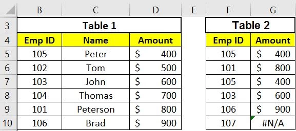
In this formula, we are using VLOOKUP to find the Salary (column 3) for each Employee ID in Table 2 by searching in the SOURCE TABLE (Table 1). The [range_lookup] is set to FALSE for an exact match.
As you can see, for Employee IDs 101, 103, 105 and 106, the corresponding Salary values are fetched correctly. However, for Employee ID 107, which is not present in Table 1, the formula returns #N/A because there is no exact match.
This way, VLOOKUP EXACT MATCH helps bring corresponding values from a source table to an output table based on an exact match of a key identifier (Employee ID in this case).
VLOOKUP Approximate Match
VLOOKUP with an APPROXIMATE MATCH is used when we want to find a value within a range. For this, we input TRUE or 1 in the [range_lookup]. When we need to find a value between two values, we use an APPROXIMATE MATCH. Let’s understand this with an example using the table below:
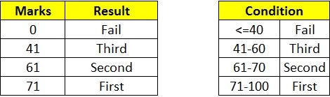
Before using APPROXIMATE MATCH, it is necessary for us to understand in which situations we can use it. For this purpose, a table has been used above for student marks, making it easier for you to comprehend. An example is illustrated in the table below.
Example:
=VLOOKUP(G15,K$14:L$18,2,TRUE)
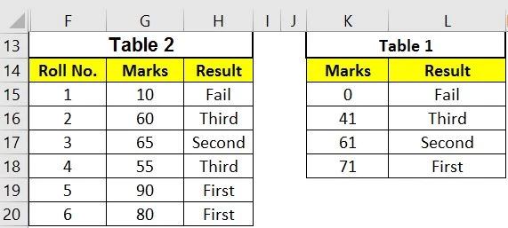
As shown in the table above, it has been demonstrated in which situations we should use APPROXIMATE MATCH and where it can be applied. For this purpose, a table has been presented for student marks. Here, we have two tables. In Table 1, the situation is defined for student marks, and APPROXIMATE MATCH is used. In Table 2, the student’s position is illustrated based on the information from Table 2.
Conclusion
I hope that in this article, you have learned to use the VLOOKUP function, and you will be able to apply it easily in Excel. If you encounter any difficulties or have any questions, please feel free to comment; we would be happy to respond to your queries. Thank you!